Models
Models
The Soil and Water Assessment Tool (SWAT) is a physically based and semi-distributed hydrological model proposed by the United States Department of Agriculture (USDA). SWAT model is used to run hydrological models to get water balance ratios like: Streamflow/Precipitation, Baseflow/Total flow, Evapotranspiration/Precipitations etc.
SWAT model was applied in Anthemountas, Mouriki and Upper Volturno-Calore basin to (i) investigate the spatiotemporal variation of runoff, groundwater recharge (RCHA), and potential evapotranspiration (PET), and (ii) quantify the groundwater depletion magnitude driven by climate variability within the three basins.
The SWAT model considers climatic information, specifically precipitation and maximum and minimum values of temperature, for the determination of the main processes involved in the hydrological cycle. Morphology, soil infiltration degree, vegetation type, and agricultural practices are also considered in the evaluation since they can greatly affect the overall groundwater balance. During the SWAT processing, the analysed basin is divided into multiple sub-basins, further subdivided into hydrologic response units (HRUs) according to the land use type, slope range, and soil units. The main step of the model consists of the creation of the HRUs, referring to all those portions of a territory characterized by unique land-use, morphological, and soil attributes combination (Figure 1). In this study, the scheme followed for groundwater balance modeling involves four steps: (1) collection of data and spatial database preparation, (2) calibration and validation, (3) comparison of the basins, and (4) interpretation of results.
The input data used for the simulation process are the following:
➢ Climatic data (daily rainfall, min and max air temperature)
➢ Soil data
➢ DEM
➢ Land Use
➢ Streamflow
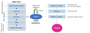
Figure 1. Project setup of SWAT model.
Primary and secondary data were jointly used in this study. Fieldwork started with a reconnaissance survey to obtain a general understanding of the hydrogeological features of the study areas, such as geological mapping and the collection of meteorological data from the stations. During the survey, data were also collected from online free access sources (Table 1) and relevant literature.
| Raw Data | Extension | Format | Reference |
| Soil Classification | World | Shapefile | http://www.fao.org/geonetwork/srv/en/metadata.show?id=14116
https://www.isric.org/explore/wosis |
| Digital Elevation Model (DEM) | World | Raster | https://asterweb.jpl.nasa.gov/gdem.asp |
| Historical climatic data | world | Database | https://www.ncei.noaa.gov/cdo-web/ |
| Land Use classification | Europe | Shapefile | https://land.copernicus.eu/pan-european/corine-land-cover |
| Climate Projections | World | Database | https://esgf-data.dkrz.de/search/esgf-dkrz/ |
| Monthly data of ET | World | Raster | https://earthdata.nasa.gov/ |
Further information about SWAT can be found at https://swat.tamu.edu/ .
Snow algorithm
The developed source code (snow_processing.py file) is written in python (https://www.python.org/), which is an interpreted high-level general-purpose programming language and is often used as a support language for software developers. The code uses as input satellite data (in a standard data netcdf format) from the NASA website (https://search.earthdata.nasa.gov/search).
All libraries and modules needed to install and run the code are open source and freely available. Generally, the majority of the modules used in Python programming are accessed by using the import statement (https://docs.python.org/3/tutorial/modules.html). The user has to define the root of the stored satellite data (dir_path) and the storage of the output files (dir_out). Once the user defines the root paths and runs the program, the code starts the processing of the data and the exporting of files. The algorithm’s outputs of Routine #1 are: (i) a csv file with written the values of the SWE and the SD in the selected areas and (ii) maps/quicklooks of the SWE for certain days, based on the selection of the user.
The output of the algorithm is then used in the second routine (Routine #2) for calculating the snow depth and for plotting the monthly/seasonal/yearly variation of the snow parameters.
Summarized below are the steps that have been applied during the processing, which consists of the following:
➢ Reading the satellite dataset and selecting the region of interest
➢ Data Screening
➢ Estimation of the spatial distribution of SWE and SD in the user selected area
➢ Calculation of the spatial distribution of the snow depth (HS) in the selected areas.
➢ Calculation of the monthly/seasonal/yearly variation of the snow parameters (SWE, HS, ρ) in the selected areas.
➢ Mapping the snow parameters in the selected areas.
Generally, the snow water equivalent (SWE) represents the amount of water that is contained in a snowpack. Using SI units, it is measured in kg/m2 , which can be considered as the weight of the meltwater per square meter that would result if the snowpack was melted entirely. Given that SWE and snow depth (HS) are derived from the satellite data, the snow density (ρ) is then calculated following the equation:
SWE = HS *ρ
Where: SWE is measured in kg/m2 , HS in m, and ρ in kg/m3
Additionally, the validation of the satellite dataset with the in-situ information is made. The relative root mean squared error (rRMSE) and the Pearson correlation coefficient are used as metrics of convergence between the satellite retrievals and the snow parameters of the reference ground-based stations. The comparison is made through the snow_comparison.py file.
This class calculates the maximum output per day that the turbine can use to generate power
The useful volume of the reservoir in relation to the height of the water in the dam and its surface is given by the equation 2.
| Equation 2 : | 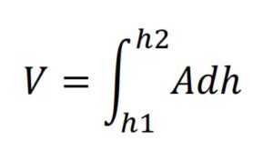 |
The current volume at any given time according to the continuity equation is the linear composition of the cumulative input curve, the cumulative output-loss curve and the cumulative consumption curve. Two restrictions are imposed on the above volume, the first concerns a minimum volume of Vmin corresponding to a level below which water is unusable for energy production. The second concerns a maximum volume of Vmax corresponding to a level beyond which the water through the dam overflow ends up at the receiver. The current volume for time T is given by equation 3.
| Equation 3 : |
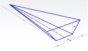
Evaporation is ignored in the model due to the small size of the reservoirs. The geometric model is the one shown in figure 1. Given that this type of dams are constructed perpendicular to the flow of small torrents, the above geometric model is quite close to reality and offers an easy and simple way of describing the useful volume with relatively little geometric data.
The function between current useful volume and change in height is calculated in Equation 4.
| Equation 4 : |
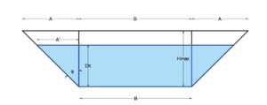
Equation 4 is a linear relationship between useful volume of water in the reservoir and change in water level. The water surface (As) and water height (Dh) curve in the reservoir is also useful. The calculation of the equation of the two variables is presented in equation 5-6 and figure 3
| Equation 5 : | 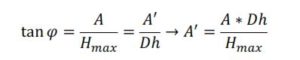 |
| Equation 6 : | 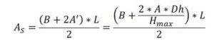 |
In the literature, the current volume curve and the reservoir surface curve are usually shown in a common diagram. For this model the diagram is presented in Figure 4.
Figure 4 reservoir level-storage curve
The current maximum and minimum water volume are also shown in Figure 5
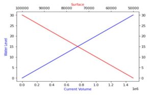
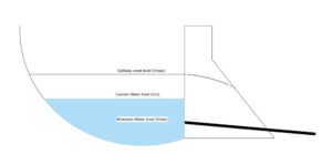
Figure 5 reservoir water’s volume
1. Optimization Model
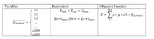
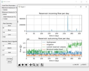
The goal of the optimization model is to find the vector of daily water supplies per year used to generate electricity. That is, the problem has 365 unknown variables. Restrictions include ensuring a minimum volume in the reservoir set at 10% of the maximum volume, ensuring a minimum irrigation supply. Also the volume of the reservoir is limited by a maximum value beyond which the excess water escapes from the overflow. The objective function is the annual energy production from the turbine. The energy production is given by equation 7.
| Equation 7 : | |
| Εurbine : The energy produced
ρ : The density of water g : The acceleration of gravity Dh : The net height of water drop Qturbine : The discharge of water
|
Based on the above the model is presented in the equations of Table 1
The model is solved by the harmony search algorithm and the whole process is organized in Python language.
GUI VERSION
flopy (MODFLOW2005) model for recharge
import numpy as np
import flopy
import itertools
# Assign name and create modflow model object
modelname = 'GrecoDam'
mf = flopy.modflow.Modflow(modelname, exe_name="mf2005")
# Model domain and grid definition
Lx = 5000.
Ly = 5000.
ztop = 100.
zbot = 0.
nlay = 1
nrow = 100
ncol = 100
delr = Lx / ncol
delc = Ly / nrow
delv = (ztop - zbot) / nlay
x_coord = np.linspace(delr/2, Lx-delr/2, num=ncol)
y_coord = np.linspace(Ly-delc/2, delc/2, num=nrow)
botm = np.linspace(ztop, zbot, nlay + 1)
hk = 1.
vka = 1.
sy = 0.1
ss = 1.e-4
laytyp = 1
# define boundary conditions: 1 everywhere except
# left and right edges, which are -1
ibound = np.ones((nlay, nrow, ncol), dtype=np.int32)
ibound[:,:,(0,ncol-1)] = -1.0
# initial conditions
strt = 80. * np.ones((nlay, nrow, ncol), dtype=np.float32)
# Time step parameters
nper = 2
perlen = [100,100]
nstp = [100,100]
steady = [False,False]
# Flopy objects
dis = flopy.modflow.ModflowDis(mf, nlay, nrow, ncol, delr=delr, delc=delc,
top=ztop, botm=botm[1:],
nper=nper, perlen=perlen, nstp=nstp, steady=steady)
bas = flopy.modflow.ModflowBas(mf, ibound=ibound, strt=strt)
lpf = flopy.modflow.ModflowLpf(mf, hk=hk, vka=vka, sy=sy, ss=ss, laytyp=laytyp)
pcg = flopy.modflow.ModflowPcg(mf)
# set up pumping well
r_well = round(nrow/2)
c_well = round(ncol/2)
wel_sp1 = [[0, r_well, c_well, -100],[0, 10, 10, -1000],[0, 20, 40, -150],[0, 30, 50, -1200],[0, 50, 50, -1900],[0, 70, 70, -2000],[0, 80, 80, -1100],[0, 80, 30, -1200],[0, 90, 90, 0],[0, 90, 10, -1800],[0, 85, 20, -1900]]
wel_sp2 = [[0, r_well, c_well, 0],[0, 10, 10, -100],[0, 20, 20, -150],[0, 30, 30, -120],[0, 50, 50, -190],[0, 70, 70, -200],[0, 80, 80, -110],[0, 80, 30, -120],[0, 90, 90, +1000],[0, 90, 10, -180],[0, 85, 20, -190]]
stress_period_data = {0: wel_sp1,
1: wel_sp2}
wel = flopy.modflow.ModflowWel(mf, stress_period_data=stress_period_data)
# Add recharge package
recharge_rate = 1e-4 # Adjust as needed
rch = flopy.modflow.ModflowRch(mf, rech=recharge_rate)
# Output control
#oc = flopy.modflow.ModflowOc(mf, save_every=True, compact=True)
oc = flopy.modflow.ModflowOc(mf, save_every=True, compact=True, stress_period_data={(0, 1): ['save head', 'save drawdown', 'save budget']})
# Write the model input files
mf.write_input()
# Run the model
success, mfoutput = mf.run_model(silent=True, pause=False, report=True)
if not success:
raise Exception('MODFLOW did not terminate normally.')
# Imports
import matplotlib.pyplot as plt
import flopy.utils.binaryfile as bf
# Create the headfile object
headobj = bf.HeadFile(modelname+'.hds', text='head')
# get data
time = headobj.get_times()[0]
head = headobj.get_data(totim=time)
extent = (x_coord[0],x_coord[ncol-1],y_coord[0],y_coord[nrow-1])
# Well point
wpt = (float(round(ncol/2)+0.5)*delr, float(round(nrow/2)+0.5)*delc)
# plot of head
plt.subplot(2,1,1)
plt.imshow(head[0,:,:], extent=extent, cmap='BrBG')
plt.colorbar()
plt.plot(wpt[0], wpt[1], lw=0, marker='o', markersize=8,
markeredgewidth=0.5,
markeredgecolor='black',
markerfacecolor='none',
zorder=9)
# cross-section (L-R) of head through the well
plt.subplot(2,1,2)
plt.plot(x_coord, head[0,r_well,:])
plt.show()
# timeseries
idx = (0, r_well, c_well)
ts = headobj.get_ts(idx)
plt.subplot(1, 1, 1)
ttl = 'Head at cell ({0},{1},{2})'.format(idx[0] + 1, idx[1] + 1, idx[2] + 1)
plt.title(ttl)
plt.xlabel('time')
plt.ylabel('head')
plt.plot(ts[:, 0], ts[:, 1])
plt.show()
import flopy.utils.postprocessing as post
# Period 1 (end of 10 years)
heads_period1 = headobj.get_data(kstpkper=(0, 0, 9))
water_table_period1 = post.get_water_table(heads_period1[0], nodata=-999.99) # Use the correct format
# Period 2 (end of 20 years)
heads_period2 = headobj.get_data(kstpkper=(0, 0, 19))
water_table_period2 = post.get_water_table(heads_period2[0], nodata=-999.99) # Use the correct format
# Contour plot for the water table at the end of the first period
plt.contour(water_table_period1, cmap='viridis', extent=(0, ncol * delc, 0, nrow * delr))
plt.title('Water Table at the end of the first period (10 years)')
plt.colorbar(label='Water Table Elevation (meters)')
plt.show()
# Contour plot for the water table at the end of the second period
plt.contour(water_table_period2, cmap='viridis', extent=(0, ncol * delc, 0, nrow * delr))
plt.title('Water Table at the end of the second period (20 years)')
plt.colorbar(label='Water Table Elevation (meters)')
plt.show()
# Plot the head versus time
idx = (0, int(nrow / 2) - 1, int(ncol / 2) - 1)
ts = headobj.get_ts(idx)
fig = plt.figure(figsize=(6, 6))
ax = fig.add_subplot(1, 1, 1)
ttl = f"Head at cell ({idx[0] + 1},{idx[1] + 1},{idx[2] + 1})"
ax.set_title(ttl)
ax.set_xlabel("time")
ax.set_ylabel("head")
ax.plot(ts[:, 0], ts[:, 1], "bo-")